The large scale stratospheric wind patterns consist of air moving upwards in the tropics and then poleward, exiting at mid- to high latitudes. There is also more rapid exchange of air between low and high latitudes (Plumb, 2002). Aerosols will be transported by these winds, and so both where they are in latitude and how long they stay in the stratosphere are affected by the stratospheric winds.
Metric
The mean lifetime of a passive tracer injected at 21km and 30°N/S is less than 2 years
Uncertainty
The inter-model variation in burden of a passive tracer across GeoMIP models is likely large (although is not quantifiable here, without some additional model experiments as described below). It is likely that a passive tracer lifetime in UKESM might sit below the 2 year cut-off defined in the metric (based on the values shown in Figure 1), but this may represent biases in this model’s transport that put it outside the plausible real world range (Figure 2).
Decision relevance
While recent models show quite consistent global cooling per unit injection, with a 4-model range of [1.0 - 1.3] °C/ 10 Mt SO2 for our central SAI scenario (Lee et al. 2026), this may be by chance. It hides strong variation in both aerosol lifetime, and in cooling per unit aerosol burden, which largely cancel out for these models. The uncertainty in transport is therefore responsible, in combination with uncertainty in aerosol size distribution, for approximately a factor of two range in the required injection magnitude to achieve a given global cooling. If lifetime of the passive tracer was well below our central estimate, as defined in the metric, this would imply a first-order increase in the required injection to achieve a given climate impact. Varying the injection magnitude could theoretically offset such differences, and this would in turn affect other impacts such as sulfur deposition. The uncertainty could therefore affect efficacy by >20%, but is unlikely to strongly influence the overall cost-benefit, resulting in a ‘medium’ decision relevance. Uncertainty in transport is potentially less important for HiLLA SAI strategies. In this case, as long as lifetime covers the first summer and is less than one year, as model simulations suggest is the case (Duffey et al., 2026), variation between, e.g., a four and eight month lifetime causes little change in climate impacts, as forcing is concentrated in the summer months. In the HiLLA case, the dominant removal mechanism is also different to low latitude SAI; quasi-horizontal mixing equatorward, and across the tropopause, is more important in this case.
Further Information
We will discuss here both our uncertainty in characterization of stratospheric winds, which arises from limited observations, and the variation and biases in the representation of those winds across earth system models. While the latter is distinct from our true ‘uncertainty’ in transport, it is an important quantity given that earth system models are our principal tool for informing decision making on SAI.
Why does it matter?
The stratospheric transport of aerosols has two primary effects:
- It changes the aerosol lifetime and therefore the amount of sunlight reflection and cooling for a given amount of injection, and;
- It changes the spatial pattern of sunlight reflection and therefore the spatial pattern of climate response, for a given injection strategy.
The lifetime of sulfate aerosols in the stratosphere (or equivalently, the burden of sulfate in the stratosphere for a given injection rate) differs by a factor of two across the most-recent GeoMIP model simulations (Lee et al., 2026; and Figure 1, below). The uncertainty in stratospheric transport does not wholly define the aerosol lifetime, since this also depends on gravitational settling of the aerosols (which increases with aerosol size). However, the inter-model variation in transport does have a strong impact on lifetime. This is demonstrated by the fact that UKESM1 has a smaller effective radius than CESM2-WACCM under the G6-1.5K-SAI simulations (and so slower gravitational settling), but approximately half the burden and lifetime (Lee et al., 2026), so the inter-model range in transport-driven lifetime variation must be at least a factor of two.
The consequence of uncertainty in transport on spatial distribution of aerosols in the horizontal plane is also important. It contributes to variation in the equator-to-pole gradients of cooling and regional climate changes under SAI (e.g. Zhang et al., 2024; Henry et al., 2024), as well as other impacts like ozone loss and sulfur deposition. However, we focus our assessment of decision-relevance here on the aerosol lifetime impact because choice of injection latitude could be used to largely offset variation in the spatial distribution (Kravitz et al., 2017).
Sources of uncertainty and state of understanding
The large-scale stratospheric transport is determined by the breaking of planetary scale Rossby waves and of small scale gravity waves. The breaking of waves moves air horizontally (or along isentropes), mixing air between higher and lower latitudes, and also deposits momentum that drives upward motion in the tropics and poleward and downward flow in the extratropics. Rossby wave breaking depends strongly on background winds, so the mean state of the stratosphere is very important (Charney and Drazin, 1961). The mean state is highly seasonally dependent, with easterly winds in the midlatitudes in summertime and westerly winds in wintertime, and thus the circulation also has a very strong seasonal cycle. Biases in the mean state of the atmosphere project quite strongly onto the stratospheric transport, and mean state biases are pervasive (e.g., Simpson et al. 2020). Gravity waves are not resolved in climate models, but are parameterized, with deleterious impact on representation of modes of variability (Achatz et al. 2024). Accurately modeling stratospheric transport is therefore a real challenge, and one for which multiple generations of climate models have not improved their performance (Abalos et al. 2026).
Explaining the metric
The burden of sulfate aerosols, as shown in Figure 1, is a useful summary of information about the lifetime of stratospheric aerosols. However, the burden (or equivalently, lifetime) is also influenced by size distribution (which controls gravitational sedimentation), so it does not isolate the circulation effects as a passive tracer would. At present, available earth system model simulations do not allow for a separation of these contributions, meaning our value of “2 years” chosen in the metric is somewhat arbitrary. Planned model experiments will simulate the evolution of such a passive tracer in order to quantify the relative impact of settling and transport on aerosol distribution under our injection scenario.
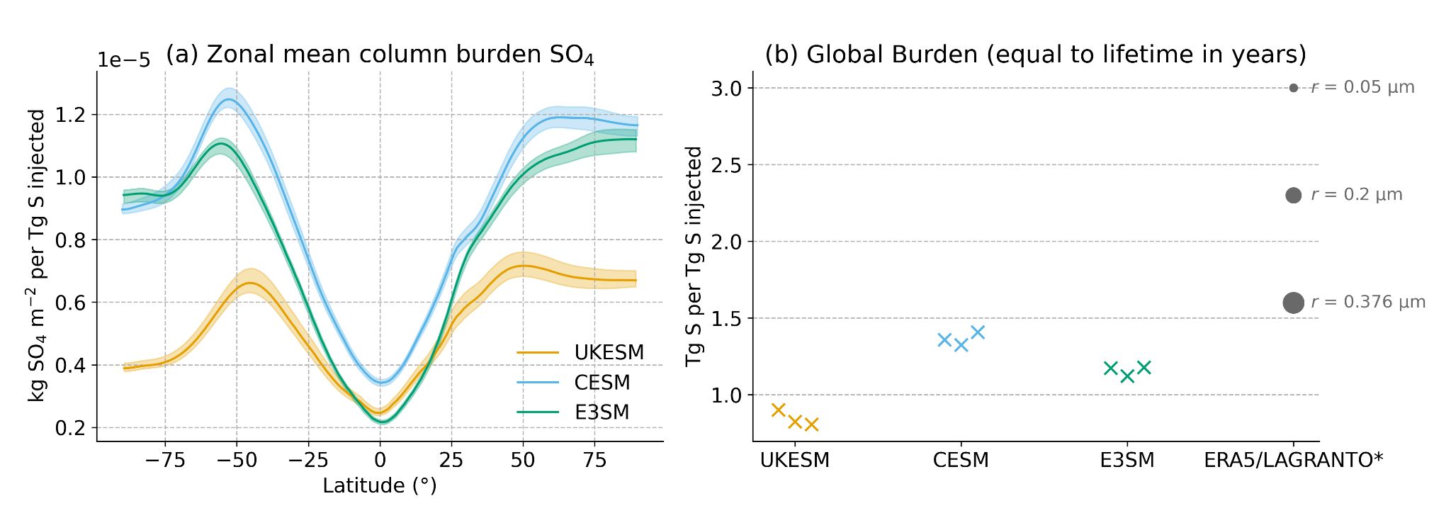
Figure 1: Zonal mean (a) and global total (b) burden of sulfate (in S per annual S injected, or equivalently, lifetime in years) under the G6-1.5K-SAI experiment in three earth system models (UKESM1.1 - ‘UKESM’, CESM2-WACCM - ‘CESM’, and E3SMv3 - ‘E3SM’), and for ERA5/LAGRANTO - a transport simulation forced with ERA5 reanalysis data. The latter data points are from Figure S1 in Sun et al. (2023), and use a different injection strategy to the other cases - still at 21km but now uniform over the tropics instead of at 30°N and 30°S. These include settling velocity for a given radius, and so there is a wide range in burden. Shaded regions are the range across the three available ensemble members, and solid lines are the ensemble means (a). Each member is plotted individually in (b). All values are time means over the final 20 years of the simulation, 2065-2084.
It is important to distinguish between our true uncertainty in aerosol transport, and biases in the model representation of this transport (relative to, for example, reanalysis products). We choose here to focus our metric on the latter because this quantity determines the model outputs which feed into decision making. An alternative metric targeting the latter might use the variation in lifetimes across Lagrangian trajectories generated from a range of reanalysis products. It is not yet clear whether this range, which is likely not small (based on age of air from reanalyses, Garny et al. 2024), would be larger or smaller than the range across current earth system models.
Describe existing modeling evidence and model observations comparisons
Summarizing from Abalos et al. (2026): Chemistry climate models disagree with observations for stratospheric transport both for the vertical transport and the horizontal mixing. For vertical velocities, the circulation is too fast, especially in boreal spring. There are significant differences between different reanalysis products, which means that there are not enough observations to constrain the stratospheric circulation. Meanwhile mixing efficiencies are too low in the most recent generation of models, though mixing is more challenging to compare with reanalysis or observations.
Another relevant comparison is how different models compare to each other and to the observations for the lifetime of volcanic aerosols. Comparisons of different models for Mt. Pinatubo reveal that the intermodel range includes the observations for sulfate burdens in the tropics, but that models consistently have too much transport into the northern hemisphere and not enough transport into the southern hemisphere (Quaglia et al. 2023).
Many recent assessments of SAI make use of a handful of ESMs, particularly UKESM1 and CESM2-WACCM. These two models, but particularly UKESM1, both have faster circulation than observed (Abalos et al., 2026), and tropopause heights biased high relative to reanalysis (Duffey et al., 2026, and Figure 2, below), suggesting that they (particularly UKESM1) may underestimate aerosol lifetimes and burdens.
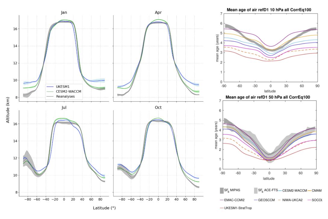
Figure 2: Left - Time-mean tropopause height over [1991-2015] under historical scenario (models) and in reanalyses. The shaded regions show the ensemble range for models, and solid lines the ensemble mean, while for reanalyses the range is over five produces (ERA5, ERA, MERRA2, NCEP, and NCEP2), as calculated by Hoffman & Spang (2022). In both cases the 1st thermal tropopause height by the WMO definition is used. Right - from Abalos et al., (2026), age-of-air in CCMI models and observations, over 1990-2010. Age of air is a measure of how long an air parcel has been in the stratosphere since it entered at the tropical tropopause. It is an Eulerian representation of the Lagrangian history of the air parcels at a given location, and therefore it is very closely related to the transport. Differences in age across different regions and gradients of age are linked to the strength of the circulation and stratospheric mixing quantitatively (Linz et al. 2016, 2021), but are frequently used somewhat more qualitatively to get a sense of how quickly air moves through the stratosphere and to evaluate differences between models and observations (Garny et al. 2024). This figure shows the age of air at 50 hPa for several models and based on satellite observations of SF6 from two independent satellite products. (For more details about the details of using SF6 as an age tracer, see Saunders et al. 2025.) This comparison shows that models have consistently younger age, which means that air is not staying in the stratosphere as long in the models as it is in reality. Note that “UKESM1-StratTrop” here is the same model version (with unified stratosphere-troposphere chemistry) as ‘UKESM1’ used for recent SAI simulations (e.g. Henry et al., 2023).
What future research is needed?
Near term research priorities include new Earth System Model experiments using passive tracers (or varying sized particles) to quantify the lifetime and distribution of aerosols without gravitational settling (or of the impact of settling across sizes), to characterize the contribution of transport alone to uncertainty in these features. Additionally, further Lagrangian trajectory simulations with multiple different reanalysis products could quantify the uncertainty in passive tracer distributions under plausible injection scenarios, given the best current knowledge of stratospheric circulation.
In the longer term, new balloon and remote sensing observations of trace gases relevant to the stratospheric circulation and improved data assimilation approaches could reduce uncertainty in our calculations of the stratospheric circulation and in reanalyses. Model improvements, such as for gravity wave parameterization or mean state biases, might reduce circulation biases that currently produce unrealistic transport in some models.
References
18Have feedback on this entry?
Spot something off, missing, or worth adding? We’d love to hear from you.
Share feedback